Tag Archives: Python

AI on the Edge LESSON 27: Track Objects of Interest in OpenCV Using Contours

AI on the Edge LESSON 27: Track Objects of Interest in OpenCV Using Contours

Hey everyone, Paul McWhorter here from TopTechBoy.com. Welcome back to our channel, where we learn to build real, intelligent systems on edge hardware. Grab yourself a nice hot cup of coffee or a cold glass of iced tea, because today we are taking a massive leap forward in our computer vision journey.

Up until now, we have learned how to configure our cameras, calculate frame rates smoothly, and isolate specific objects based on color using the HSV color space. We built beautiful masks and composite images that show only our target color. But let’s be honest with ourselves: a mask is just a collection of white pixels on a black screen. The computer doesn’t actually know where the object is, how big it is, or how to follow it if it moves.

In this lesson, we are going to fix that. We are going to teach the machine to look at our mask, isolate the single biggest shape of interest, ignore the background noise, and draw a real-time bounding tracking box around it. This is true object tracking.

The Core Concept: What is a Contour?

Think of a contour as a mathematical boundary line. When OpenCV looks at a binary mask (where your target object is white and everything else is black), a contour is the continuous line that traces the outer edge of that white shape.

The beauty of contours is that they turn a chaotic cloud of thousands of isolated pixels into structured, manageable vector shapes. Once OpenCV finds these shapes, it can calculate their physical properties, such as their area, perimeter, and exact center.

The Three Steps to Algorithmic Object Tracking

To turn a raw camera frame into a fully tracked target, our script follows a strict three-part engineering pipeline inside our main execution loop:

1. Extracting Every Boundary

First, we pass our binary mask into OpenCV’s contour detection engine. We configure it to use external retrieval, meaning it will ignore any hollow holes inside the object and only trace the outermost boundary. It returns a list of every single contour it finds in the frame.

2. Hunting for the Largest Target

In the real world, your camera view is never perfectly clean. Even with an excellent HSV color mask, you will get random speckles, reflections, or background noise showing up as tiny white dots on your mask. If we tried to track everything, our program would lose its mind. To solve this, we use a Python maximization function to scan our list of contours and extract the absolute largest one based on its physical area.

3. Setting an Area Noise Floor

Even after finding the largest contour, what happens if your object completely leaves the camera view? The largest remaining “object” might be a tiny, single-pixel spec of static noise on the edge of the screen. To prevent our tracking box from jumping around erratically, we establish a strict structural threshold—a noise floor. If the area of the largest contour isn’t big enough to confidently be our target, we ignore it completely.

Drawing the Bounding Box

Once we have successfully isolated our valid, large contour, we don’t just want to draw a messy, squiggly line around it. We want clean coordinates that an automation system or a robotic pan-tilt kit could actually use to follow the target.

We pass our largest contour into a bounding rectangle function. OpenCV automatically calculates the exact mathematical limits of that shape and returns four precise numbers:

    • X: The horizontal starting pixel coordinate of the object.

    • Y: The vertical starting pixel coordinate of the object.

    • W: The total width of the object in pixels.

    • H: The total height of the object in pixels.

With those four dimensions locked down, we use a standard drawing function to overlay a crisp, green rectangle directly onto our live color camera feed. Now, as you move your object around the room, the box follows it dynamically, tracking its position in real time at high frame rates.

Note you will have to tune the LC and UC parameters for your object of interest, as we showed last week.


AI on the Edge LESSON 26: Understanding the HSV Color Space in OpenCV

Hey guys, welcome back to the channel. If you’ve been following along, you know we’ve been pushing our hardware absolutely down into the dirt. We’ve been running large language models right on the edge, pushing our boards hot and heavy until the silicon is screaming and the thermal throttling flags are popping up all over the place.

But today, we are stepping away from the heavy-compute server terminals, and we are getting back to our roots: Real-Time Computer Vision and Embedded Control. In our previous lessons, we learned how to hook up our high-speed camera, capture raw frames, and interact with individual pixels using standard RGB/BGR math. But today, we are going to look under the hood of a completely different way of representing color: The HSV Color Space (Hue, Saturation, Value).

If you try to track objects or isolate specific colors in the traditional RGB world, you are going to pull your hair out. The moment a shadow hits your object or the room lighting changes, your Red, Green, and Blue values completely collapse. By shifting our mathematics into the HSV space, we can lock onto a color’s pure identity regardless of whether it is sitting under a bright laboratory spotlight or a dim shadow.

Not only are we going to capture and process these video streams at a smooth-as-silk 60 frames per second, but we are also going to translate that raw visual math directly into the physical world. We are using our trusty SunFounder Fusion HAT+ to dynamically pulse an external RGB LED, matching its brightness and color hue perfectly to whatever pixel your mouse is clicking on in real-time.

Let’s look at the blueprint to make this happen.

The Complete Python Code

Here is the clean, un-guardrailed Python script for today’s lesson. Paste this directly into your local terminal workspace. No bloated libraries, no unnecessary frameworks—just pure, deliberate engineering.

Under the Hood: How the Code Works

1. The Real-Time Telemetry Smooth Filter

Look closely at how we calculate our frames-per-second metric inside the main processing loop:

If you simply print out the raw math of 1 / deltaT, your numbers on the screen are going to jump all over the place like a wild animal. By applying a 95% historical weight and a 5% instant weight, we create a low-pass software filter that smoothly tracks our true hardware operational speed without erratic layout jitter.

2. The Mouse Vector and BGR Array Sequence

When your mouse triggers an event over the window, OpenCV passes us the standard coordinate pairs (x, y). But remember: inside a NumPy data structure, images are structured as Rows first, then Columns. That means when you slice into your image array to read a pixel’s color values, you must pass the parameters as frame[y, x]. If you pass it as [x, y], your program is going to index out of bounds and crash hard.

Furthermore, always remember that OpenCV handles colors in a BGR (Blue, Green, Red) sequence, not RGB. When we extract those elements, they unpack straight into valB, valG, valR.

3. Masking and Bitwise Isolation

To lock onto our target color, we use cv2.inRange() to look at our HSV frame and check it against our lower constraint (LC) and upper constraint (UC). This generates a Mask—a pure black-and-white image where pixels within the target color space are completely white (255), and everything else is completely black (0).

By taking that mask and running a fast bitwise operation

We force the computer to evaluate every single pixel. If the mask is zero, the output is blacked out. If the mask is active, the original, rich color information passes through perfectly, isolating our target object from the background noise instantly.

Get your circuits wired up, get this script running on your machine, and let me know in the comments section below what kind of performance numbers you are pulling on your local workbench. I’ll catch you guys in the next lesson!

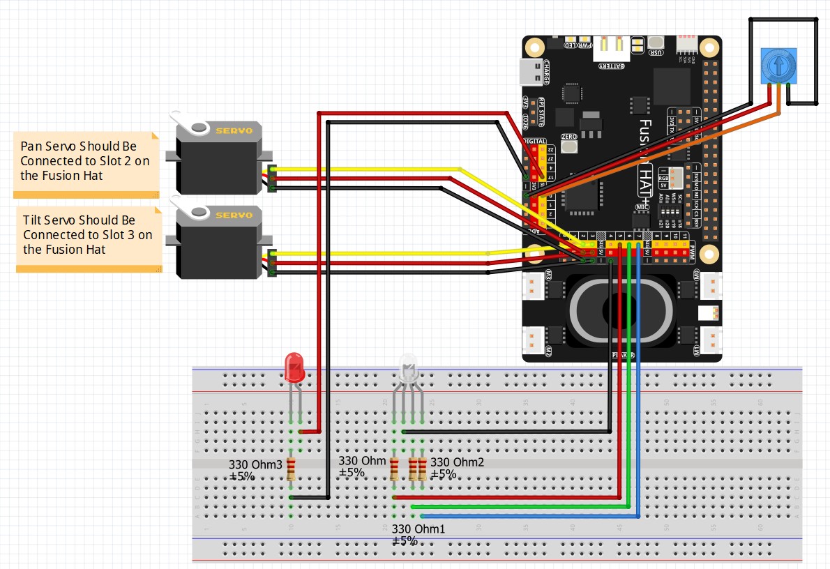
Remember we are still setting the LED color to the color that cursor is pointing at. This is the circuit for connecting the RGB LED.

Fusion Hat Circuit Diagram
This is the circuit we will use moving forward in the class

AI on the Edge LESSON 25: Create Region of Interest (ROI) in openCV Using the Mouse

Well, hello there! I’m absolutely delighted you could join me today. If you’ve been following along with our journey into AI on the Edge, you know that we are getting closer and closer to building some truly powerful, real-world computer vision applications. But before we can get to the fancy AI stuff, we have to master the fundamentals. Today, we’re tackling something that is going to make your projects look—and feel—a whole lot more professional: creating a Region of Interest (ROI) using the mouse.

Why Do We Need an ROI?

Think about it. When you’re processing a video feed, you’re usually wasting a ton of compute power looking at things that don’t matter. Maybe you’re tracking a ball on a table, but your camera is seeing the whole room. Why process the walls and the ceiling when you only care about the table? By defining an ROI, we tell our code: “Ignore everything else. Only look here.” It saves processing time, it reduces noise, and it makes your AI much more accurate.

Interacting with OpenCV

In this lesson, we’re going to step beyond simple static code. I’m going to show you how to use OpenCV’s callback functions to make your program “live.” We’ll use the mouse to click and drag a rectangle directly on the video feed to define our ROI in real-time. It’s interactive, it’s intuitive, and it’s a vital skill for anyone building real-world vision systems.

The Code

Now, I’ve put a lot of work into making this code clean and easy to follow. You’ll see exactly how we capture those mouse events—cv2.EVENT_LBUTTONDOWN, cv2.EVENT_MOUSEMOVE, and cv2.EVENT_LBUTTONUP—to create that bounding box dynamically.

Putting It to the Test

I want you to take this code, run it on your Jetson, and play around with it. Try defining different regions. Notice how the frame rate stays steady because we aren’t bogging down the CPU with unnecessary pixels. This is the “Edge” part of “AI on the Edge”—making smart, efficient decisions right where the data is being captured.

I can’t wait to see what you build with this. As always, keep those questions coming, stay curious, and most importantly—don’t get discouraged! We’re doing hard things, and you are doing a great job.

I’ll see you in the next lesson!

What questions do you have about implementing ROI in your own computer vision projects? Post them in comments on the video! Thanks for learning.

We will be using the circuit used in the earlier lessons:

Fusion Hat Circuit Diagram
This is the circuit we will use moving forward in the class


AI on the Edge LESSON 23: Creating Regions of Interest (ROI) in OpenCV with Slicing

Welcome back, everyone! In this lesson, we are stepping into a foundational aspect of computer vision: manipulation of specific regions within a video frame.

Up to this point, we have been grabbing the full frame from our camera and performing operations on the entire image. But in real-world edge AI and robotics applications, processing every single pixel of a high-resolution frame is an absolute waste of compute power. If you want to detect a license plate, track a face, or monitor a specific sensor layout on a machine, you don’t need to look at the sky or the floor. You need to isolate a Region of Interest (ROI).

In this lesson, you will learn how to use Python’s powerful matrix slicing capabilities to chop up a frame, isolate specific quadrants, manipulate pixels inside an ROI, and display multiple synchronized windows across your desktop without crashing your system footprint.

The Core Concept: Image Slicing and ROIs

In OpenCV, an image frame isn’t just a visual picture—it is a standard NumPy array. A color frame is a 3D matrix structured by rows, columns, and color channels: [Rows, Columns, Channels] or [Height, Width, Color].

Because it is a standard array, we can use standard Python slicing notation to isolate any rectangular box we want:

ROI = frame[rowstart : rowend,  colstart : colend]

The .copy() Trap

When you slice a piece of an array in Python like ROI = frame[0:100, 0:100], Python does not create a new image in your RAM. It creates a view or a pointer back to the original frame. If you modify pixels inside that ROI, you will accidentally alter your original main camera frame!

To isolate a region and modify it independently without bleeding back into your primary frame, you must explicitly use the .copy() method:

Below is the complete code script we built during the video tutorial. Copy this code exactly into your Python environment, verify your geometry setups, and run it.

Homework Assignment

Alright, it is time to earn your stripes and see if you can fly with the big dogs. Your homework assignment is to take this foundation and build a dynamic tracking target box using the array geometry principles we just learned.

  1. Create a single main camera window (640 x 360).

  2. Draw an independent rectangular ROI box that starts directly in the dead center of the screen.

  3. Using your keyboard parameters (cv2.waitKey), program the system so that using the Arrow Keys (or ‘i’, ‘j’, ‘k’, ‘l’) smoothly updates variables to move the ROI box dynamically around the screen in real-time.

  4. Crucial Constraint: Do not let your boundary indices drift off the array! You must write conditional boundaries so that if your moving target hits the edge of your $640 \times 360$ boundary layout, it locks at the frame border and prevents an out-of-bounds index crash.

  5. In a separate output window, display only the contents of the moving target box in real-time grayscaled format.

Grab your morning coffee, fire up your code editor, write the script from scratch, and do not copy-paste code you don’t understand. Leave a link to your homework solution video in the YouTube comments section so I can see your progress!

AI on the Edge LESSON 21: Managing Multiple Windows in OpenCV on the Raspberry Pi

Hey everyone, Paul McWhorter here!

Welcome back to the AI on the Edge series!

In today’s lesson, we’re going to take an important next step in computer vision. We’re going to learn how to create, position, resize, and manage multiple windows at the same time using OpenCV on the Raspberry Pi.

This might sound simple, but it’s actually a very big deal. Once you can comfortably work with multiple windows, you can start building much more powerful vision applications — like having a main camera view, a processed view, zoomed-in sections, and debug windows all running at once.

In this lesson we create:

  • One large main camera window
  • A smaller color preview
  • A small grayscale version
  • Five tiny grayscale windows stacked on the side

This gives you a clean, organized workspace while the camera is running.


What You Learned in This Lesson

  • How to create multiple named windows with cv2.namedWindow()
  • How to resize windows using cv2.resizeWindow()
  • How to precisely position windows on your screen with cv2.moveWindow()
  • How to work with different resolutions of the same image (full size, half size, quarter size)
  • Converting between color and grayscale while running live video
  • Keeping everything running smoothly with good FPS

Mastering multiple windows is one of those foundational skills that separates basic OpenCV projects from more professional and useful vision systems.


Pro Tip: Play around with the window positions and sizes after you get it working. Try making one window much larger, or experiment with different layouts. This is your workspace — make it comfortable!


Ready for the next step? In the next lesson, we’re going to start doing something really cool — we’ll begin combining live video with drawn graphics and start creating interactive vision projects.

Keep building, keep learning, and I’ll see you in the next video!

In the lesson, we develop the code below: