Tag Archives: Edge AI

The code below shows the work we did in this lesson.

AI on the Edge Lesson 37: Using RTSP and IP Cameras in OpenCV on Raspberry Pi 5

Hey guys! Welcome back to our AI on the Edge series. In our previous lessons, we’ve had a blast working with standard USB webcams, but if you are building a real-world computer vision application, an automation rig, or a security monitoring setup around your home or farm, USB cables just aren’t going to cut it. You need to pull video feeds from remote IP cameras using the Real-Time Streaming Protocol (RTSP).

Today, we are taking that exact step on the Raspberry Pi 5, connecting to an IP camera, streaming the feed smoothly into OpenCV, and—most importantly—solving the dreaded latency problem that plagues RTSP feeds.

The Big Challenge: Conquering RTSP Latency

If you’ve ever tried pulling an RTSP stream into OpenCV straight out of the box, you’ve probably noticed something frustrating: the video lags behind real-time, sometimes by several seconds or even tens of seconds.

Why does that happen? Because by default, FFmpeg and OpenCV buffer incoming frames to ensure smooth playback. But when you are doing computer vision, AI inferencing, or real-time tracking on the edge, you don’t want old history—you want right now.

To fix that, we pass the cv2.CAP_FFMPEG backend flag and immediately flush the buffer by setting the property to 0. This forces OpenCV to drop the backlog and grab the absolute newest frame available from the camera stream, keeping your Pi 5 processing live data in real-time.

Understanding the Script Structure

Let’s break down the key parts of today’s implementation:

Credentials & Resolution: We import a separate secret file to keep our camera IP addresses, usernames, and passwords safe and out of public repositories. We lock our resolution at 1280×720 to balance crisp detail with the Pi 5’s processing overhead.
Smooth FPS Calculation: Instead of a jittery raw frame-rate readout, we use an exponential moving average to give us a stable, readable performance metric on screen.
The Display Window: We configure a GUI window using OpenCV’s window flags so we can easily position and resize our output feed on the desktop.

Drop Your Questions Below

Working with network streams can sometimes be tricky depending on your specific camera’s firmware, codec settings, and network stability. If you run into any connection drops or lag spikes on your Raspberry Pi 5, drop a comment on the video!

Keep building, stay creative, and I will see you guys in Lesson 38!

Here is the code developed in the video

# ====================================================================
# DISCLAIMER:
# This code is provided as-is for educational and experimental 
# purposes only. The author makes no representations or warranties of 
# any kind concerning the safety, suitability, or accuracy of this 
# code. Use at your own risk. The author assumes no liability for any 
# damages, system failures, security breaches, or network issues 
# resulting from the use or implementation of this script.
# ====================================================================
import cv2
import time
import secret
W=1280
H=720
tStart = time.time()
fps = 0
RES = (W,H)

textLowerLeft = (int(W*.01),int(H*.05))
fontFace = cv2.FONT_HERSHEY_SIMPLEX
fontThickness = int(W/425)
fontScale = H*.0015
fontColor = (0,0,255)
print(secret.RTSP8)
cam = cv2.VideoCapture(secret.RTSP1, cv2.CAP_FFMPEG)
cam.set(cv2.CAP_PROP_BUFFERSIZE, 0)
cam.set(cv2.CAP_PROP_POS_FRAMES, 0)

cv2.namedWindow('Camera',cv2.WINDOW_GUI_NORMAL)
cv2.moveWindow('Camera',0,65)
cv2.resizeWindow('Camera',W,H)

while True:
    deltaT = time.time() - tStart
    tStart=time.time()
    fps = fps*.95 + (1/deltaT)*.05
    _, frame= cam.read()
    #frame=cv2.flip(frame,-1)
    myText = "FPS: "+str(round(fps,1))
    cv2.putText(frame,myText,textLowerLeft,fontFace,fontScale,fontColor,fontThickness)
    cv2.imshow("Camera", frame)
    if cv2.waitKey(1)==ord('q'):
        break
cv2.destroyAllWindows()
print('Program Terminated')

# ====================================================================

# DISCLAIMER:

# This code is provided as-is for educational and experimental

# purposes only. The author makes no representations or warranties of

# any kind concerning the safety, suitability, or accuracy of this

# code. Use at your own risk. The author assumes no liability for any

# damages, system failures, security breaches, or network issues

# resulting from the use or implementation of this script.

# ====================================================================

import cv2

import time

import secret

W=1280

H=720

tStart = time.time()

fps = 0

RES = (W,H)

textLowerLeft = (int(W*.01),int(H*.05))

fontFace = cv2.FONT_HERSHEY_SIMPLEX

fontThickness = int(W/425)

fontScale = H*.0015

fontColor = (0,0,255)

print(secret.RTSP8)

cam = cv2.VideoCapture(secret.RTSP1, cv2.CAP_FFMPEG)

cam.set(cv2.CAP_PROP_BUFFERSIZE, 0)

cam.set(cv2.CAP_PROP_POS_FRAMES, 0)

cv2.namedWindow('Camera',cv2.WINDOW_GUI_NORMAL)

cv2.moveWindow('Camera',0,65)

cv2.resizeWindow('Camera',W,H)

while True:

deltaT = time.time() - tStart

tStart=time.time()

fps = fps*.95 + (1/deltaT)*.05

_, frame= cam.read()

#frame=cv2.flip(frame,-1)

myText = "FPS: "+str(round(fps,1))

cv2.putText(frame,myText,textLowerLeft,fontFace,fontScale,fontColor,fontThickness)

cv2.imshow("Camera", frame)

if cv2.waitKey(1)==ord('q'):

break

cv2.destroyAllWindows()

print('Program Terminated')

NVIDIA, NVIDIA Jetson Orin Nano

Local Voice Control of NVIDIA Jetson Orin Nano with STT: Getting Started with Vosk

July 22, 2026 admin

Engineering Your Own Local Voice Assistant: No Cloud, No Compromise

Most “smart” voice assistants are just glorified remote controls for someone else’s server. Today, we’re changing that. We are going to build a local, offline voice command pipeline. This isn’t just about saving data; it’s about ownership. When you can control your hardware—like opening and closing a farm gate—without an internet connection, you have built a system that is robust, private, and yours to control forever. Today you are going to get Speech to Text up and running on your NVIDIA Jetson Orin Nano running under Jetpack 7.2.

The “Why” Behind the Setup

You might ask, “Why not just use a cloud API?” Because cloud APIs are fragile. They rely on internet stability, external servers, and privacy-invasive data logging. By running Vosk locally, we keep the processing on your hardware (like the NVIDIA Jetson). It’s faster, it works in the middle of a power-isolated homestead, and it’s 100% secure.

Part 1: Preparing the Environment

Before we can make the machine listen, we have to prepare the battlefield. We aren’t just downloading files; we are setting up a stable environment where your dependencies won’t conflict with your OS.

# Create a dedicated directory so our work stays organized
mkdir -p ~/STT
cd ~/STT

# We need the PortAudio headers. Why? Because Python’s 'pyaudio' is just a wrapper.
# Under the hood, it talks to the C-based PortAudio library. If the headers aren't there,
# the library won't compile, and your microphone will never wake up.
sudo apt update
sudo apt install -y portaudio19-dev wget unzip

# Download the lightweight, low-latency English model weights from Vosk
wget https://alphacephei.com/vosk/models/vosk-model-small-en-us-0.15.zip

# Unzip the archive and rename the folder cleanly to 'model' so the Python script finds it
unzip vosk-model-small-en-us-0.15.zip
mv vosk-model-small-en-us-0.15 model

# Clean up the downloaded zip file to keep the folder pristine
rm vosk-model-small-en-us-0.15.zip

# Setting up a Virtual Environment (venv) is the hallmark of a pro.
# It traps our project dependencies inside this folder so we don't break our system Python.
python3 -m venv sttVenv
source sttVenv/bin/activate
pip install --upgrade pip

# Vosk does the heavy lifting for speech recognition, and Pyaudio grabs the raw data.
pip install vosk pyaudio

# Create a dedicated directory so our work stays organized

mkdir -p ~/STT

cd ~/STT

# We need the PortAudio headers. Why? Because Python’s 'pyaudio' is just a wrapper.

# Under the hood, it talks to the C-based PortAudio library. If the headers aren't there,

# the library won't compile, and your microphone will never wake up.

sudo apt update

sudo apt install -y portaudio19-dev wget unzip

# Download the lightweight, low-latency English model weights from Vosk

wget https://alphacephei.com/vosk/models/vosk-model-small-en-us-0.15.zip

# Unzip the archive and rename the folder cleanly to 'model' so the Python script finds it

unzip vosk-model-small-en-us-0.15.zip

mv vosk-model-small-en-us-0.15 model

# Clean up the downloaded zip file to keep the folder pristine

rm vosk-model-small-en-us-0.15.zip

# Setting up a Virtual Environment (venv) is the hallmark of a pro.

# It traps our project dependencies inside this folder so we don't break our system Python.

python3 -m venv sttVenv

source sttVenv/bin/activate

pip install --upgrade pip

# Vosk does the heavy lifting for speech recognition, and Pyaudio grabs the raw data.

pip install vosk pyaudio

This is IMPORTANT!

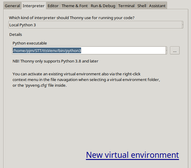
Now you can post the code below. You also have to point Thonny to run in the virtual environment. Open Thonny, and under run – select interpreter. Then you must point it to /home/yourUserName/STT/ttsVenv/bin/python3. For me, my username is pjm, but you put in your user name in path above. Here is what mine looked like:

Part 2: Solving the PipeWire Challenge

The biggest headache in modern Linux audio is PipeWire. If you try to open a microphone stream using a hardcoded sample rate that doesn’t match your hardware, your program won’t just fail—it will segfault. We use the validation script below to programmatically query the hardware, asking it: “What sample rate are you running at?” before we even try to open a stream.

# Import the PyAudio library to handle real-time microphone recording and audio stream manipulation.
import pyaudio
# Import the built-in JSON module to parse the structured text results returned by the speech recognition engine.
import json
# Import the audioop library to perform real-time mathematical operations and downsampling on raw audio byte data.
import audioop
# Import the core Vosk objects: Model loads the AI brain/weights, and KaldiRecognizer handles the acoustic processing.
from vosk import Model, KaldiRecognizer
# Import the standard OS module to reliably build absolute system file paths across different user directories.
import os
state=None

# Define a function to discover the specific hardware index and sample rate of the active system sound server.
def get_pipewire_index():
    # Instantiate a PyAudio session object to query the operating system's hardware configuration list.
    p = pyaudio.PyAudio()
    # Loop through every single available audio device reported by the operating system kernel.
    for i in range(p.get_device_count()):
        # Retrieve a descriptive configuration dictionary for the current audio device index.
        dev = p.get_device_info_by_index(i)
        # Check if the name of the device contains 'pipewire' to target the modern Linux audio subsystem.
        if "pipewire" in dev.get('name', '').lower():
            # Return the valid device index integer and its hardware default sample rate, converted cleanly to an integer.
            return i, int(dev.get('defaultSampleRate'))
    # Return empty values if the loop completes without finding an active PipeWire sound server profile.
    return None, None

# Execute the discovery function to capture both the correct system hardware device index and its native sample rate.
dev_index, native_rate = get_pipewire_index()

# Check if the hardware discovery handshake failed to locate an active PipeWire audio interface.
if dev_index is None:
    # Alert the user on screen that the script cannot communicate with the system's active audio server layer.
    print("Error: Could not find 'pipewire' device.")
    # Stop the script execution immediately since it is impossible to record audio without a valid device hook.
    exit()

# Instantiate a fresh PyAudio session specifically dedicated to opening our incoming recording channel.
p = pyaudio.PyAudio()
# Open the active system recording stream channel using explicit audio hardware parameter configurations.
# PARAMETER MANUAL:
# - format=pyaudio.paInt16: Sets 16-bit Signed Integer PCM format. (LEAVE ALONE - required by the Vosk engine).
# - channels=1: Sets recording to Mono channel audio. (LEAVE ALONE - Vosk processes single-channel input).
# - rate=native_rate: Sets the sample rate to match the mic exactly. (LEAVE ALONE - prevents driver hardware failure).
# - input=True: Configures this stream as an audio capture device. (LEAVE ALONE - required to wake up the microphone).
# - input_device_index=dev_index: Points to our discovered target device. (LEAVE ALONE - ensures we grab the right mic).
# - frames_per_buffer=4096: Controls audio chunk size. (PLAY WITH: Lower values like 2048 reduce latency but risk buffer overflows; higher values like 8192 increase safety but introduce slight latency).
stream = p.open(format=pyaudio.paInt16, channels=1, rate=native_rate, 
                input=True, input_device_index=dev_index, frames_per_buffer=4096)

# Generate an absolute directory path targeting the exact folder containing your extracted acoustic model weights.
# PARAMETER MANUAL:
# - "STT", "model": Represents folder names. (PLAY WITH: Change these only if your physical folder layout uses different names).
model_path = os.path.join(os.path.expanduser("~"), "STT", "model")
# Load the heavy machine learning weights into system memory to initialize the Vosk voice processing brain.
model = Model(model_path)
# Initialize the primary speech recognizer object using the loaded model weights and target processing frequency.
# PARAMETER MANUAL:
# - model: The initialized AI brain variable. (LEAVE ALONE).
# - 16000: Specifies the target processing sample rate in Hertz. (LEAVE ALONE - Vosk models are mathematically trained for exactly 16000Hz).
recognizer = KaldiRecognizer(model, 16000)

# Print a status message to the terminal showing that the handshake succeeded and revealing the mic's operating frequency.
print(f"Listening on PipeWire at {native_rate}Hz...")
# Turn on the hardware recording valve to begin filling up the system input data buffers.
stream.start_stream()

# Set up an exception safety block to intercept manual user exits gracefully without leaving system resources locked up.
try:
    # Launch the infinite real-time audio capture loop to continuously monitor the microphone stream.
    while True:
        # Pull raw binary audio frame bytes directly out of the incoming hardware stream buffer memory block.
        # PARAMETER MANUAL:
        # - 4096: The chunk size to read. (LEAVE ALONE - must perfectly match your stream's frames_per_buffer setting).
        # - exception_on_overflow=False: Prevents Python crashes if the Orin momentarily falls behind. (LEAVE ALONE).
        data = stream.read(4096, exception_on_overflow=False)
        # Downsample the raw audio bytes mathematically to 16000Hz using digital filtering algorithms.
        # PARAMETER MANUAL:
        # - data: Raw input audio byte string. (LEAVE ALONE).
        # - 2: Size of sample width in bytes for 16-bit sound. (LEAVE ALONE).
        # - 1: Input audio channel count. (LEAVE ALONE).
        # - native_rate: The native frequency of your mic. (LEAVE ALONE).
        # - 16000: The required downsampled output frequency. (LEAVE ALONE).
        # - state: The digital filtering conversion state history object. (LEAVE ALONE).
        # CRITICAL NOTE: The 'state' variable must be initialized as 'state = None' before entering this 'try:' block, 
        # otherwise Python will throw a NameError on the very first loop iteration because 'state' does not exist yet.
        data_16k, state = audioop.ratecv(data, 2, 1, native_rate, 16000, state)
        
        # Feed the processed 16kHz audio data block into Vosk to evaluate if a complete spoken phrase has finished.
        if recognizer.AcceptWaveform(data_16k):
            # Parse the structured JSON text string returned by the acoustic model into a standard Python dictionary.
            res = json.loads(recognizer.Result())
            # Check the parsed result dictionary to ensure that the detected text sequence is not completely blank.
            if res.get("text"):
                # Cleanly output the decoded text command straight to the standard system terminal display screen.
                print("Command: "+res['text'])
# Intercept the user pressing Ctrl+C in the terminal to stop the continuous script loop cleanly.
except KeyboardInterrupt:
    # Print a clean closing status notification on a new line to confirm the signal was intercepted.
    print("\nStopped.")
# Execute mandatory clean up instructions that are guaranteed to run no matter how the script terminates or crashes.
finally:
    # Turn off the active recording stream data valve to stop pulling raw information from the audio driver layer.
    stream.stop_stream()
    # Close the recording stream channel completely to drop the active hardware pointer binding handles.
    stream.close()
    # Terminate the parent PyAudio engine instance to release all allocated audio device resources back to the OS.
    p.terminate()

100

101

102

103

104

105

106

107

108

# Import the PyAudio library to handle real-time microphone recording and audio stream manipulation.

import pyaudio

# Import the built-in JSON module to parse the structured text results returned by the speech recognition engine.

import json

# Import the audioop library to perform real-time mathematical operations and downsampling on raw audio byte data.

import audioop

# Import the core Vosk objects: Model loads the AI brain/weights, and KaldiRecognizer handles the acoustic processing.

from vosk import Model, KaldiRecognizer

# Import the standard OS module to reliably build absolute system file paths across different user directories.

import os

state=None

# Define a function to discover the specific hardware index and sample rate of the active system sound server.

def get_pipewire_index():

# Instantiate a PyAudio session object to query the operating system's hardware configuration list.

p = pyaudio.PyAudio()

# Loop through every single available audio device reported by the operating system kernel.

for i in range(p.get_device_count()):

# Retrieve a descriptive configuration dictionary for the current audio device index.

dev = p.get_device_info_by_index(i)

# Check if the name of the device contains 'pipewire' to target the modern Linux audio subsystem.

if "pipewire" in dev.get('name', '').lower():

# Return the valid device index integer and its hardware default sample rate, converted cleanly to an integer.

return i, int(dev.get('defaultSampleRate'))

# Return empty values if the loop completes without finding an active PipeWire sound server profile.

return None, None

# Execute the discovery function to capture both the correct system hardware device index and its native sample rate.

dev_index, native_rate = get_pipewire_index()

# Check if the hardware discovery handshake failed to locate an active PipeWire audio interface.

if dev_index is None:

# Alert the user on screen that the script cannot communicate with the system's active audio server layer.

print("Error: Could not find 'pipewire' device.")

# Stop the script execution immediately since it is impossible to record audio without a valid device hook.

exit()

# Instantiate a fresh PyAudio session specifically dedicated to opening our incoming recording channel.

p = pyaudio.PyAudio()

# Open the active system recording stream channel using explicit audio hardware parameter configurations.

# PARAMETER MANUAL:

# - format=pyaudio.paInt16: Sets 16-bit Signed Integer PCM format. (LEAVE ALONE - required by the Vosk engine).

# - channels=1: Sets recording to Mono channel audio. (LEAVE ALONE - Vosk processes single-channel input).

# - rate=native_rate: Sets the sample rate to match the mic exactly. (LEAVE ALONE - prevents driver hardware failure).

# - input=True: Configures this stream as an audio capture device. (LEAVE ALONE - required to wake up the microphone).

# - input_device_index=dev_index: Points to our discovered target device. (LEAVE ALONE - ensures we grab the right mic).

# - frames_per_buffer=4096: Controls audio chunk size. (PLAY WITH: Lower values like 2048 reduce latency but risk buffer overflows; higher values like 8192 increase safety but introduce slight latency).

stream = p.open(format=pyaudio.paInt16, channels=1, rate=native_rate,

input=True, input_device_index=dev_index, frames_per_buffer=4096)

# Generate an absolute directory path targeting the exact folder containing your extracted acoustic model weights.

# PARAMETER MANUAL:

# - "STT", "model": Represents folder names. (PLAY WITH: Change these only if your physical folder layout uses different names).

model_path = os.path.join(os.path.expanduser("~"), "STT", "model")

# Load the heavy machine learning weights into system memory to initialize the Vosk voice processing brain.

model = Model(model_path)

# Initialize the primary speech recognizer object using the loaded model weights and target processing frequency.

# PARAMETER MANUAL:

# - model: The initialized AI brain variable. (LEAVE ALONE).

# - 16000: Specifies the target processing sample rate in Hertz. (LEAVE ALONE - Vosk models are mathematically trained for exactly 16000Hz).

recognizer = KaldiRecognizer(model, 16000)

# Print a status message to the terminal showing that the handshake succeeded and revealing the mic's operating frequency.

print(f"Listening on PipeWire at {native_rate}Hz...")

# Turn on the hardware recording valve to begin filling up the system input data buffers.

stream.start_stream()

# Set up an exception safety block to intercept manual user exits gracefully without leaving system resources locked up.

try:

# Launch the infinite real-time audio capture loop to continuously monitor the microphone stream.

while True:

# Pull raw binary audio frame bytes directly out of the incoming hardware stream buffer memory block.

# PARAMETER MANUAL:

# - 4096: The chunk size to read. (LEAVE ALONE - must perfectly match your stream's frames_per_buffer setting).

# - exception_on_overflow=False: Prevents Python crashes if the Orin momentarily falls behind. (LEAVE ALONE).

data = stream.read(4096, exception_on_overflow=False)

# Downsample the raw audio bytes mathematically to 16000Hz using digital filtering algorithms.

# PARAMETER MANUAL:

# - data: Raw input audio byte string. (LEAVE ALONE).

# - 2: Size of sample width in bytes for 16-bit sound. (LEAVE ALONE).

# - 1: Input audio channel count. (LEAVE ALONE).

# - native_rate: The native frequency of your mic. (LEAVE ALONE).

# - 16000: The required downsampled output frequency. (LEAVE ALONE).

# - state: The digital filtering conversion state history object. (LEAVE ALONE).

# CRITICAL NOTE: The 'state' variable must be initialized as 'state = None' before entering this 'try:' block,

# otherwise Python will throw a NameError on the very first loop iteration because 'state' does not exist yet.

data_16k, state = audioop.ratecv(data, 2, 1, native_rate, 16000, state)

# Feed the processed 16kHz audio data block into Vosk to evaluate if a complete spoken phrase has finished.

if recognizer.AcceptWaveform(data_16k):

# Parse the structured JSON text string returned by the acoustic model into a standard Python dictionary.

res = json.loads(recognizer.Result())

# Check the parsed result dictionary to ensure that the detected text sequence is not completely blank.

if res.get("text"):

# Cleanly output the decoded text command straight to the standard system terminal display screen.

print("Command: "+res['text'])

# Intercept the user pressing Ctrl+C in the terminal to stop the continuous script loop cleanly.

except KeyboardInterrupt:

# Print a clean closing status notification on a new line to confirm the signal was intercepted.

print("\nStopped.")

# Execute mandatory clean up instructions that are guaranteed to run no matter how the script terminates or crashes.

finally:

# Turn off the active recording stream data valve to stop pulling raw information from the audio driver layer.

stream.stop_stream()

# Close the recording stream channel completely to drop the active hardware pointer binding handles.

stream.close()

# Terminate the parent PyAudio engine instance to release all allocated audio device resources back to the OS.

p.terminate()

Homework: Your Gate Controller

You now have a system that identifies audio input, resamples it to 16kHz, and outputs text. Your assignment: Transform this text output into an action.

I want you to add a conditional statement to the main loop. If the recognized text is “open”, print an ASCII art representation of an open gate. If it’s “close”, print the closed version. This is the first step in closing the loop between your AI and the physical world. Go get ’em, and don’t just copy the code—understand how the data flows from the microphone to your decision logic!

AI On the Edge, Raspberry Pi

AI on the Edge LESSON 33: Tracking Faces with Pan Tilt Camera in OpenCV on Pi 5

July 16, 2026 admin

Hey guys, Paul McWhorter here from toptechboy.com. In today’s lesson, we are taking our “AI on the Edge” skills to the next level. We aren’t just detecting faces anymore; we are going to make our camera system react to them.

We are integrating our computer vision logic with physical hardware to create a pan-tilt tracking system. We’ll use the Raspberry Pi 5 to run high-speed inference, detect a face, calculate exactly how far that face has drifted from the center of our frame, and then command our servos to follow it in real-time. It is one thing to see a box draw around a face; it is a completely different level of “cool” when the camera actually turns to look at you.

The Engineering Concept: The Error Loop

In robotics, this is a classic control problem. We have a Target (the center of the face) and a Setpoint (the center of our camera frame). The difference between these two points is our Error.

xError: How far left or right the face is from the center.
yError: How far up or down the face is from the center.

By taking that error and dividing it by a “gain” constant (in our case, 50/2), we can smoothly adjust the servo angles. If we don’t divide by a constant, the camera will snap aggressively to the target or overshoot it. This simple division creates a “proportional” response that keeps our tracking smooth and precise.

What to Focus On

Make sure you have your picamera2 and fusion_hat libraries updated and configured before you dive in. The key to this lesson isn’t just getting the servos to move—it’s understanding how to bridge the gap between the coordinates returned by OpenCV and the angle coordinates required by your servo library.

Pay close attention to how we calculate the center of the frame and the center of the detected face box. Once you understand that math, you can use this same logic to track anything: faces, colored objects, or even specific shapes!

Homework Assignment: Show Your Work!

Alright guys, no excuses! If you want to truly master this hardware, you cannot just sit there and watch me do it—you have to write the code and run it yourself.

Your Task: Get this tracking system working. Once you have it tracking a face, I want you to experiment with that “Gain” factor (the 50/2 part). Try increasing it and decreasing it. What happens to the tracking quality? Is it smoother? Does it jitter?

Record a video of your camera following your face around the room, upload it to YouTube, and link back to this video at the top of your page. Post a link to your homework in the comments section below so I can see you running your code like a boss.

The code we developed in the video is available below.

# ====================================================================
# DISCLAIMER:
# This code is provided as-is for educational and experimental 
# purposes only. The author makes no representations or warranties of 
# any kind concerning the safety, suitability, or accuracy of this 
# code. Use at your own risk. The author assumes no liability for any 
# damages, system failures, security breaches, or network issues 
# resulting from the use or implementation of this script.
# ====================================================================
 
import cv2
import time
from picamera2 import Picamera2
from fusion_hat.servo import Servo
panPin = 2
tiltPin = 3
panServo = Servo(panPin)
tiltServo = Servo(tiltPin)
panAngle = -10
tiltAngle =-20
panServo.angle(panAngle)
tiltServo.angle(tiltAngle)
piCam = Picamera2()
W=1280
H=720
tStart = time.time()
fps = 0
RES = (W,H)
piCam.preview_configuration.main.size = RES
piCam.preview_configuration.main.format = "RGB888"
piCam.preview_configuration.controls.FrameRate=60
piCam.preview_configuration.align()
piCam.configure("preview")
piCam.start()

textLowerLeft = (int(W*.01),int(H*.05))
fontFace = cv2.FONT_HERSHEY_SIMPLEX
fontThickness = int(W/425)
fontScale = H*.0015
fontColor = (0,0,255)

faceFinder = cv2.CascadeClassifier(cv2.data.haarcascades + 'haarcascade_frontalface_default.xml')
eyeFinder = cv2.CascadeClassifier(cv2.data.haarcascades + "haarcascade_eye.xml")

track = False
xFrameC = int((W-1)/2)
yFrameC = int((H-1)/2)
xBoxC = xFrameC
yBoxC = yFrameC

def mouseAction(event, x, y, flags, param):
    global frame, track
    if event == 0:
        xPos = x
        yPos = y
    if frame is not None:
        frameHSV = cv2.cvtColor(frame, cv2.COLOR_BGR2HSV)
        Hue, Sat, Val = frameHSV[y,x]
        if Hue == 60:
            track = True
        if Hue == 0:
            track = False
cv2.namedWindow('Camera',cv2.WINDOW_GUI_NORMAL)
cv2.moveWindow('Camera',0,65)
cv2.resizeWindow('Camera',W,H)
cv2.setMouseCallback('Camera',mouseAction)

while True:
    deltaT = time.time() - tStart
    tStart=time.time()
    fps = fps*.95 + (1/deltaT)*.05
    frame= piCam.capture_array()
    frame=cv2.flip(frame,-1)
    
    cv2.circle(frame,(int(.9*W),int(.1*H)),20,(0,255,0),-1)
    cv2.circle(frame, (int(.95*W),int(.1*H)),20,(0,0,255),-1)

    gray = cv2.cvtColor(frame,cv2.COLOR_BGR2GRAY)
    faces = faceFinder.detectMultiScale(gray,scaleFactor=1.1, minNeighbors =5, minSize=(100,100))
    for (x,y,w,h) in faces:
        cv2.rectangle(frame, (x,y),(x+w,y+h),(0,255,255),3)
        
        xBoxC = x + int(w/2)
        yBoxC = y + int(h/2)
        xError = xBoxC - xFrameC
        yError = yBoxC - yFrameC
        
        eyes =eyeFinder.detectMultiScale(gray[y:y+h,x:x+w],scaleFactor=1.1,minNeighbors=5,minSize=(15,15))
        for (i,j,w,h) in eyes:
            cv2.rectangle(frame,(x+i,y+j),(x+i+w,y+j+h),(255,0,0),3)
    
    if track == True and len(faces)>0:
        panAngle = panAngle - xError/50/2
        panServo.angle(int(panAngle))
        #time.sleep(.02)
        tiltAngle = tiltAngle + yError/50/2
        tiltServo.angle(int(tiltAngle))
        #time.sleep(.02)
                        
    
    myText = "FPS: "+str(round(fps,1))
    cv2.putText(frame,myText,textLowerLeft,fontFace,fontScale,fontColor,fontThickness)
    cv2.imshow("Camera", frame)
    cv2.moveWindow("Camera",0,60)
    if cv2.waitKey(1)==ord('q'):
        break
cv2.destroyAllWindows()
print('Program Terminated')

100

101

102

103

104

105

106

107

108

# ====================================================================

# DISCLAIMER:

# This code is provided as-is for educational and experimental

# purposes only. The author makes no representations or warranties of

# any kind concerning the safety, suitability, or accuracy of this

# code. Use at your own risk. The author assumes no liability for any

# damages, system failures, security breaches, or network issues

# resulting from the use or implementation of this script.

# ====================================================================

import cv2

import time

from picamera2 import Picamera2

from fusion_hat.servo import Servo

panPin = 2

tiltPin = 3

panServo = Servo(panPin)

tiltServo = Servo(tiltPin)

panAngle = -10

tiltAngle =-20

panServo.angle(panAngle)

tiltServo.angle(tiltAngle)

piCam = Picamera2()

W=1280

H=720

tStart = time.time()

fps = 0

RES = (W,H)

piCam.preview_configuration.main.size = RES

piCam.preview_configuration.main.format = "RGB888"

piCam.preview_configuration.controls.FrameRate=60

piCam.preview_configuration.align()

piCam.configure("preview")

piCam.start()

textLowerLeft = (int(W*.01),int(H*.05))

fontFace = cv2.FONT_HERSHEY_SIMPLEX

fontThickness = int(W/425)

fontScale = H*.0015

fontColor = (0,0,255)

faceFinder = cv2.CascadeClassifier(cv2.data.haarcascades + 'haarcascade_frontalface_default.xml')

eyeFinder = cv2.CascadeClassifier(cv2.data.haarcascades + "haarcascade_eye.xml")

track = False

xFrameC = int((W-1)/2)

yFrameC = int((H-1)/2)

xBoxC = xFrameC

yBoxC = yFrameC

def mouseAction(event, x, y, flags, param):

global frame, track

if event == 0:

xPos = x

yPos = y

if frame is not None:

frameHSV = cv2.cvtColor(frame, cv2.COLOR_BGR2HSV)

Hue, Sat, Val = frameHSV[y,x]

if Hue == 60:

track = True

if Hue == 0:

track = False

cv2.namedWindow('Camera',cv2.WINDOW_GUI_NORMAL)

cv2.moveWindow('Camera',0,65)

cv2.resizeWindow('Camera',W,H)

cv2.setMouseCallback('Camera',mouseAction)

while True:

deltaT = time.time() - tStart

tStart=time.time()

fps = fps*.95 + (1/deltaT)*.05

frame= piCam.capture_array()

frame=cv2.flip(frame,-1)

cv2.circle(frame,(int(.9*W),int(.1*H)),20,(0,255,0),-1)

cv2.circle(frame, (int(.95*W),int(.1*H)),20,(0,0,255),-1)

gray = cv2.cvtColor(frame,cv2.COLOR_BGR2GRAY)

faces = faceFinder.detectMultiScale(gray,scaleFactor=1.1, minNeighbors =5, minSize=(100,100))

for (x,y,w,h) in faces:

cv2.rectangle(frame, (x,y),(x+w,y+h),(0,255,255),3)

xBoxC = x + int(w/2)

yBoxC = y + int(h/2)

xError = xBoxC - xFrameC

yError = yBoxC - yFrameC

eyes =eyeFinder.detectMultiScale(gray[y:y+h,x:x+w],scaleFactor=1.1,minNeighbors=5,minSize=(15,15))

for (i,j,w,h) in eyes:

cv2.rectangle(frame,(x+i,y+j),(x+i+w,y+j+h),(255,0,0),3)

if track == True and len(faces)>0:

panAngle = panAngle - xError/50/2

panServo.angle(int(panAngle))

#time.sleep(.02)

tiltAngle = tiltAngle + yError/50/2

tiltServo.angle(int(tiltAngle))

#time.sleep(.02)

myText = "FPS: "+str(round(fps,1))

cv2.putText(frame,myText,textLowerLeft,fontFace,fontScale,fontColor,fontThickness)

cv2.imshow("Camera", frame)

cv2.moveWindow("Camera",0,60)

if cv2.waitKey(1)==ord('q'):

break

cv2.destroyAllWindows()

print('Program Terminated')

NVIDIA

NVIDIA Jetson Orin Nano: Secret to Running Ollama on the GPU

June 18, 2026 admin

One of the biggest frustrations with the new Jetpack 7.2 release is finding out that a standard installation of Ollama—the gold standard for running local LLMs—completely ignores your powerful NVIDIA GPU and defaults to the CPU.

In this lesson, we aren’t just going to fix that; we are going to measure the “truth” behind the performance. We will use data to see exactly how much gain we get from the GPU and where the hardware starts to hit the thermal throttling wall.

The Problem: The “Canned” Installation

When you run a standard Ollama install on the Jetson Orin Nano, the system doesn’t automatically recognize the integrated GPU (iGPU). If you open your NVIDIA Power GUI (jtop), you will see your CPU cores pegged at 100% while the GPU sits idle. This leads to slow response times and a disappointing experience.

Lets start by the standard ‘Canned’ Installation. The good news is, it is very simple:

curl -fsSL https://ollama.com/install.sh | sh

1	curl -fsSL https://ollama.com/install.sh \| sh

To see exactly how your system is performing, run Ollama in verbose mode:

ollama run gemma3:1b

1	ollama run gemma3:1b

At this point you will have Ollama running a simple LLM locally on your Jetson Orin Nano. This is a huge step forward, but we now want to dig deeper and actually see how well this simple model is performing. The first thing we do is run the Jetson Power GUI, hidden behind the NVIDIA icon in upper right of the menu bar.

Pay close attention to the Prompt Eval Rate and Eval Rate (tokens per second). These are our baseline numbers.

The “Secret Sauce” Solution

To force Ollama to use the Jetson’s CUDA cores, we have to manually override the system service configuration.

sudo apt-get update && sudo apt-get install nano

1	sudo apt-get update && sudo apt-get install nano

Step 1: Install the Nano Editor

Before we can edit system files, we need a reliable text editor. If you don’t have it yet, run this command:

Step 2: Create the Service Override

We need to tell the Ollama service exactly where to look for the GPU libraries. Use nano to open the following file:

sudo nano /etc/systemd/system/ollama.service.d/override.conf

1	sudo nano /etc/systemd/system/ollama.service.d/override.conf

Step 3: Add the Configuration

Copy and paste the following block into that file. This is the “Secret Sauce” that enables the iGPU and points the system to the correct CUDA backend:

[Service]
Environment="OLLAMA_HOST=127.0.0.1:11434"
Environment="OLLAMA_CONTEXT_LENGTH=4096"
Environment="OLLAMA_IGPU_ENABLE=1"
Environment="GGML_BACKEND_PATH=/usr/local/lib/ollama/cuda_v13/libggml-cuda.so"
Environment="LD_LIBRARY_PATH=/usr/local/lib/ollama:/usr/local/lib/ollama/cuda_v13"

[Service]

Environment="OLLAMA_HOST=127.0.0.1:11434"

Environment="OLLAMA_CONTEXT_LENGTH=4096"

Environment="OLLAMA_IGPU_ENABLE=1"

Environment="GGML_BACKEND_PATH=/usr/local/lib/ollama/cuda_v13/libggml-cuda.so"

Environment="LD_LIBRARY_PATH=/usr/local/lib/ollama:/usr/local/lib/ollama/cuda_v13"

Note: Save the file by pressing Ctrl+O, Enter, and then Ctrl+X to exit.

Step 4: Reboot

For the changes to take effect, We will do a reboot.

Benchmarking the Results

Once you have the GPU engaged, the real work begins. In the video, we look at a side-by-side comparison of performance across different Jetson Power Modes (10W, 15W, and MaxN).

Power Level	Prompt Eval Rate (t/s)	Eval Rate (t/s)	Throttling Observed?
CPU	[Your Data]	[Your Data]	Yes/No
10W	[Your Data]	[Your Data]	Yes/No
15W	[Your Data]	[Your Data]	Yes/No
MaxN	[Your Data]	[Your Data]	Yes/No

As we discovered, moving to the GPU provides a boost, but it also increases the heat signature. Watch the full video to see the charts and understand which power level provides the best “sweet spot” for stable, long-term AI performance on your Jetson Orin Nano. This is an important first step . . . getting the heavy lifting down to the GPU. Now in future videos we will explore how to get the work done Well on the GPU.

AI On the Edge, Raspberry Pi

AI on the Edge LESSON 25: Create Region of Interest (ROI) in openCV Using the Mouse

June 17, 2026 admin

Well, hello there! I’m absolutely delighted you could join me today. If you’ve been following along with our journey into AI on the Edge, you know that we are getting closer and closer to building some truly powerful, real-world computer vision applications. But before we can get to the fancy AI stuff, we have to master the fundamentals. Today, we’re tackling something that is going to make your projects look—and feel—a whole lot more professional: creating a Region of Interest (ROI) using the mouse.

Why Do We Need an ROI?

Think about it. When you’re processing a video feed, you’re usually wasting a ton of compute power looking at things that don’t matter. Maybe you’re tracking a ball on a table, but your camera is seeing the whole room. Why process the walls and the ceiling when you only care about the table? By defining an ROI, we tell our code: “Ignore everything else. Only look here.” It saves processing time, it reduces noise, and it makes your AI much more accurate.

Interacting with OpenCV

In this lesson, we’re going to step beyond simple static code. I’m going to show you how to use OpenCV’s callback functions to make your program “live.” We’ll use the mouse to click and drag a rectangle directly on the video feed to define our ROI in real-time. It’s interactive, it’s intuitive, and it’s a vital skill for anyone building real-world vision systems.

The Code

Now, I’ve put a lot of work into making this code clean and easy to follow. You’ll see exactly how we capture those mouse events—cv2.EVENT_LBUTTONDOWN, cv2.EVENT_MOUSEMOVE, and cv2.EVENT_LBUTTONUP—to create that bounding box dynamically.

# ====================================================================
# DISCLAIMER:
# This code is provided as-is for educational and experimental 
# purposes only. The author makes no representations or warranties of 
# any kind concerning the safety, suitability, or accuracy of this 
# code. Use at your own risk. The author assumes no liability for any 
# damages, system failures, security breaches, or network issues 
# resulting from the use or implementation of this script.
# ====================================================================
 
import cv2
import time
from picamera2 import Picamera2
from fusion_hat.pwm import PWM
piCam = Picamera2()
W=1280
H=720
tStart = time.time()
fps = 0

redPin = 5
greenPin = 6
bluePin = 7
redLED = PWM(redPin)
greenLED = PWM(greenPin)
blueLED = PWM(bluePin)

RES = (W,H)
piCam.preview_configuration.main.size = RES
piCam.preview_configuration.main.format = "RGB888"
piCam.preview_configuration.controls.FrameRate=60
piCam.preview_configuration.align()
piCam.configure("preview")
piCam.start()

textLowerLeft = (int(W*.01),int(H*.06))
fontFace = cv2.FONT_HERSHEY_SIMPLEX
fontThickness = int(W/425)
fontScale = H*.0015
fontColor = (0,0,255)

textLowerLeft1 = (int(W*.01),int(H*.06)*2)
textLowerLeft2 = (int(W*.01),int(H*.06)*3)
xPos = 0
yPos = 0
valR = 0
valG = 0
valB = 0
frame = None

drawing = False
startX = 0
endX = 0
makeROI = False

boxColor = (0,255,255)
boxThick = 3

def mouseAction(event, x, y, flags, param):
    global frame, xPos, yPos, valR, valG, valB
    global drawing, makeROI, startX, startY, endX, endY
    if event == 0:
        xPos = x
        yPos = y
        if frame is not None:
            valB, valG, valR = frame[y,x]
            redLED.pulse_width_percent(int(valR/255*100))
            greenLED.pulse_width_percent(int(valG/255*100/2))
            blueLED.pulse_width_percent(int(valB/255*100/4))
        if drawing == True:
            endX = x
            endY = y
    if event == 1:
        drawing = True
        makeROI = False
        startX = x
        startY = y
        endX = x
        endY = y 
    if event == 4:
        drawing = False
        makeROI = True
        endX = x
        endY = y
    
cv2.namedWindow('Camera')
cv2.moveWindow('Camera',0,65)
cv2.setMouseCallback('Camera',mouseAction)

print("Click and Drag to Draw a Box")
print("Release Mouse to Finalize box. Press q to Quit")

while True:
    deltaT = time.time() - tStart
    tStart=time.time()
    fps = fps*.95 + (1/deltaT)*.05
    frame= piCam.capture_array()
    frame=cv2.flip(frame,-1)
    
    if drawing == True:
        cv2.rectangle(frame,(startX,startY),(endX,endY),boxColor,boxThick)
    
    if makeROI == True:
        ROI = frame[startY:endY,startX:endX]
        ROIgray = cv2.cvtColor(ROI,cv2.COLOR_BGR2GRAY)
        cv2.imshow("ROI",ROI)
        cv2.imshow("ROIgray",ROIgray)
        cv2.moveWindow("ROI",W,65)
        cv2.moveWindow("ROIgray",W,endY-startY+200)
    
    myText = "FPS: "+str(round(fps,1))
    cv2.putText(frame,myText,textLowerLeft,fontFace,fontScale,fontColor,fontThickness)
    
    text1 = "Mouse Pos: "+str((xPos,yPos))
    text2 = "Pixel Color: "+str((valR,valG,valB))
    cv2.putText(frame,text1,textLowerLeft1,fontFace,fontScale,fontColor,fontThickness)    
    cv2.putText(frame,text2,textLowerLeft2,fontFace,fontScale,fontColor,fontThickness)    
    cv2.imshow("Camera", frame)
    cv2.moveWindow("Camera",0,60)
    if cv2.waitKey(1)==ord('q'):
        break
cv2.destroyAllWindows()
redLED.pulse_width_percent(0)
greenLED.pulse_width_percent(0)
blueLED.pulse_width_percent(0)
print('Program Terminated')

100

101

102

103

104

105

106

107

108

109

110

111

112

113

114

115

116

117

118

119

120

121

122

123

124

125

126

# ====================================================================

# DISCLAIMER:

# This code is provided as-is for educational and experimental

# purposes only. The author makes no representations or warranties of

# any kind concerning the safety, suitability, or accuracy of this

# code. Use at your own risk. The author assumes no liability for any

# damages, system failures, security breaches, or network issues

# resulting from the use or implementation of this script.

# ====================================================================

import cv2

import time

from picamera2 import Picamera2

from fusion_hat.pwm import PWM

piCam = Picamera2()

W=1280

H=720

tStart = time.time()

fps = 0

redPin = 5

greenPin = 6

bluePin = 7

redLED = PWM(redPin)

greenLED = PWM(greenPin)

blueLED = PWM(bluePin)

RES = (W,H)

piCam.preview_configuration.main.size = RES

piCam.preview_configuration.main.format = "RGB888"

piCam.preview_configuration.controls.FrameRate=60

piCam.preview_configuration.align()

piCam.configure("preview")

piCam.start()

textLowerLeft = (int(W*.01),int(H*.06))

fontFace = cv2.FONT_HERSHEY_SIMPLEX

fontThickness = int(W/425)

fontScale = H*.0015

fontColor = (0,0,255)

textLowerLeft1 = (int(W*.01),int(H*.06)*2)

textLowerLeft2 = (int(W*.01),int(H*.06)*3)

xPos = 0

yPos = 0

valR = 0

valG = 0

valB = 0

frame = None

drawing = False

startX = 0

endX = 0

makeROI = False

boxColor = (0,255,255)

boxThick = 3

def mouseAction(event, x, y, flags, param):

global frame, xPos, yPos, valR, valG, valB

global drawing, makeROI, startX, startY, endX, endY

if event == 0:

xPos = x

yPos = y

if frame is not None:

valB, valG, valR = frame[y,x]

redLED.pulse_width_percent(int(valR/255*100))

greenLED.pulse_width_percent(int(valG/255*100/2))

blueLED.pulse_width_percent(int(valB/255*100/4))

if drawing == True:

endX = x

endY = y

if event == 1:

drawing = True

makeROI = False

startX = x

startY = y

endX = x

endY = y

if event == 4:

drawing = False

makeROI = True

endX = x

endY = y

cv2.namedWindow('Camera')

cv2.moveWindow('Camera',0,65)

cv2.setMouseCallback('Camera',mouseAction)

print("Click and Drag to Draw a Box")

print("Release Mouse to Finalize box. Press q to Quit")

while True:

deltaT = time.time() - tStart

tStart=time.time()

fps = fps*.95 + (1/deltaT)*.05

frame= piCam.capture_array()

frame=cv2.flip(frame,-1)

if drawing == True:

cv2.rectangle(frame,(startX,startY),(endX,endY),boxColor,boxThick)

if makeROI == True:

ROI = frame[startY:endY,startX:endX]

ROIgray = cv2.cvtColor(ROI,cv2.COLOR_BGR2GRAY)

cv2.imshow("ROI",ROI)

cv2.imshow("ROIgray",ROIgray)

cv2.moveWindow("ROI",W,65)

cv2.moveWindow("ROIgray",W,endY-startY+200)

myText = "FPS: "+str(round(fps,1))

cv2.putText(frame,myText,textLowerLeft,fontFace,fontScale,fontColor,fontThickness)

text1 = "Mouse Pos: "+str((xPos,yPos))

text2 = "Pixel Color: "+str((valR,valG,valB))

cv2.putText(frame,text1,textLowerLeft1,fontFace,fontScale,fontColor,fontThickness)

cv2.putText(frame,text2,textLowerLeft2,fontFace,fontScale,fontColor,fontThickness)

cv2.imshow("Camera", frame)

cv2.moveWindow("Camera",0,60)

if cv2.waitKey(1)==ord('q'):

break

cv2.destroyAllWindows()

redLED.pulse_width_percent(0)

greenLED.pulse_width_percent(0)

blueLED.pulse_width_percent(0)

print('Program Terminated')

Putting It to the Test

I want you to take this code, run it on your Jetson, and play around with it. Try defining different regions. Notice how the frame rate stays steady because we aren’t bogging down the CPU with unnecessary pixels. This is the “Edge” part of “AI on the Edge”—making smart, efficient decisions right where the data is being captured.

I can’t wait to see what you build with this. As always, keep those questions coming, stay curious, and most importantly—don’t get discouraged! We’re doing hard things, and you are doing a great job.

I’ll see you in the next lesson!

What questions do you have about implementing ROI in your own computer vision projects? Post them in comments on the video! Thanks for learning.

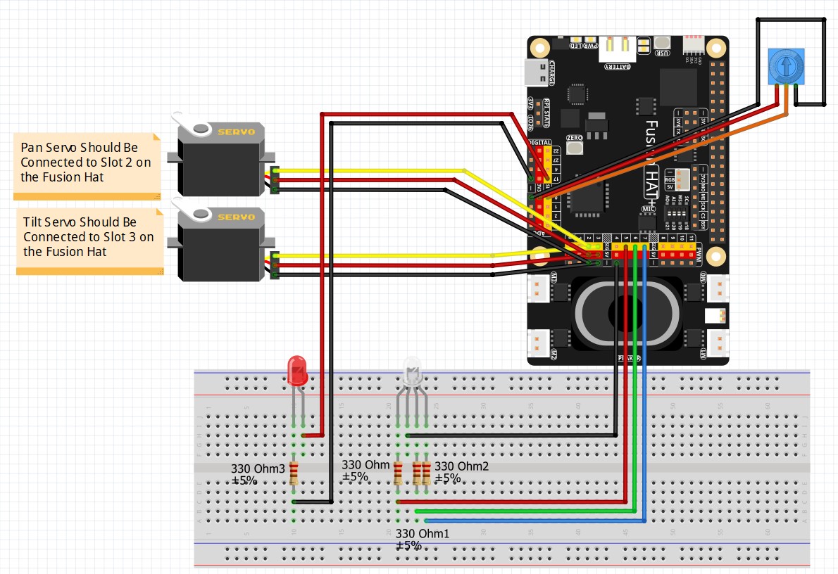
We will be using the circuit used in the earlier lessons:

Fusion Hat Circuit Diagram — This is the circuit we will use moving forward in the class

Technology Tutorials

Tag Archives: Edge AI

AI on the Edge LESSON 37: Using RTSP and IP Cameras in OpenCV on Raspberry Pi 5

AI on the Edge Lesson 37: Using RTSP and IP Cameras in OpenCV on Raspberry Pi 5

The Big Challenge: Conquering RTSP Latency

Understanding the Script Structure

Drop Your Questions Below

Local Voice Control of NVIDIA Jetson Orin Nano with STT: Getting Started with Vosk

Engineering Your Own Local Voice Assistant: No Cloud, No Compromise

The “Why” Behind the Setup

Part 1: Preparing the Environment

This is IMPORTANT!

Part 2: Solving the PipeWire Challenge

Homework: Your Gate Controller

AI on the Edge LESSON 33: Tracking Faces with Pan Tilt Camera in OpenCV on Pi 5

The Engineering Concept: The Error Loop

What to Focus On

Homework Assignment: Show Your Work!

NVIDIA Jetson Orin Nano: Secret to Running Ollama on the GPU

The Problem: The “Canned” Installation

The “Secret Sauce” Solution

Step 1: Install the Nano Editor

Step 2: Create the Service Override

Step 3: Add the Configuration

Step 4: Reboot

Benchmarking the Results

AI on the Edge LESSON 25: Create Region of Interest (ROI) in openCV Using the Mouse

Why Do We Need an ROI?

Interacting with OpenCV

The Code

Putting It to the Test

Making The World a Better Place One High Tech Project at a Time. Enjoy!