
Tag Archives: AI on the Edge

AI on the Edge LESSON 50: Control NeoPixel Ring With Hand Gestures and MediaPipe

Hey everybody, welcome back to AI on the Edge! In Lesson 50 we’re taking things to the next level — we’re combining real-time hand tracking with a physical NeoPixel ring so you can change colors just by pointing at the screen! Using MediaPipe on the Raspberry Pi, we track your index finger tip and turn the big camera view into an interactive color picker. Hover over any of the seven big colored circles (Red, Green, Blue, Cyan, Magenta, Yellow, or Black) and — boom — the NeoPixel ring instantly lights up with that color!
This lesson is super fun because it finally brings together everything we’ve been building: smooth hand detection, coordinate mapping between camera and OLED, visual feedback, and real-world hardware control. You’ll see your finger tracked with a big blue dot, watch the selected color update live on both the screen and the OLED, and control actual RGB lights with nothing but a gesture.
By the end of this lesson you’ll have a working gesture-controlled color mixer that feels like real interactive magic. This is the kind of project that makes people say “Wow, you built that on a Raspberry Pi?!”
This is also a perfect foundation for even cooler future projects — gesture-controlled lighting, touchless interfaces, interactive games, or even a full gesture-controlled robot or light show.
So grab your Raspberry Pi, hook up that NeoPixel ring, fire up the camera, and let’s start waving our hands around like we’re casting spells! As always, the complete code is right below the video. Watch along, run the code, then start tweaking it — maybe add more colors, make the ring react differently to gestures, or combine it with the hand connection drawing from earlier lessons.I’m really excited to see what you create with this one!Now go make something awesome! 

This is the core circuit we use for the class:
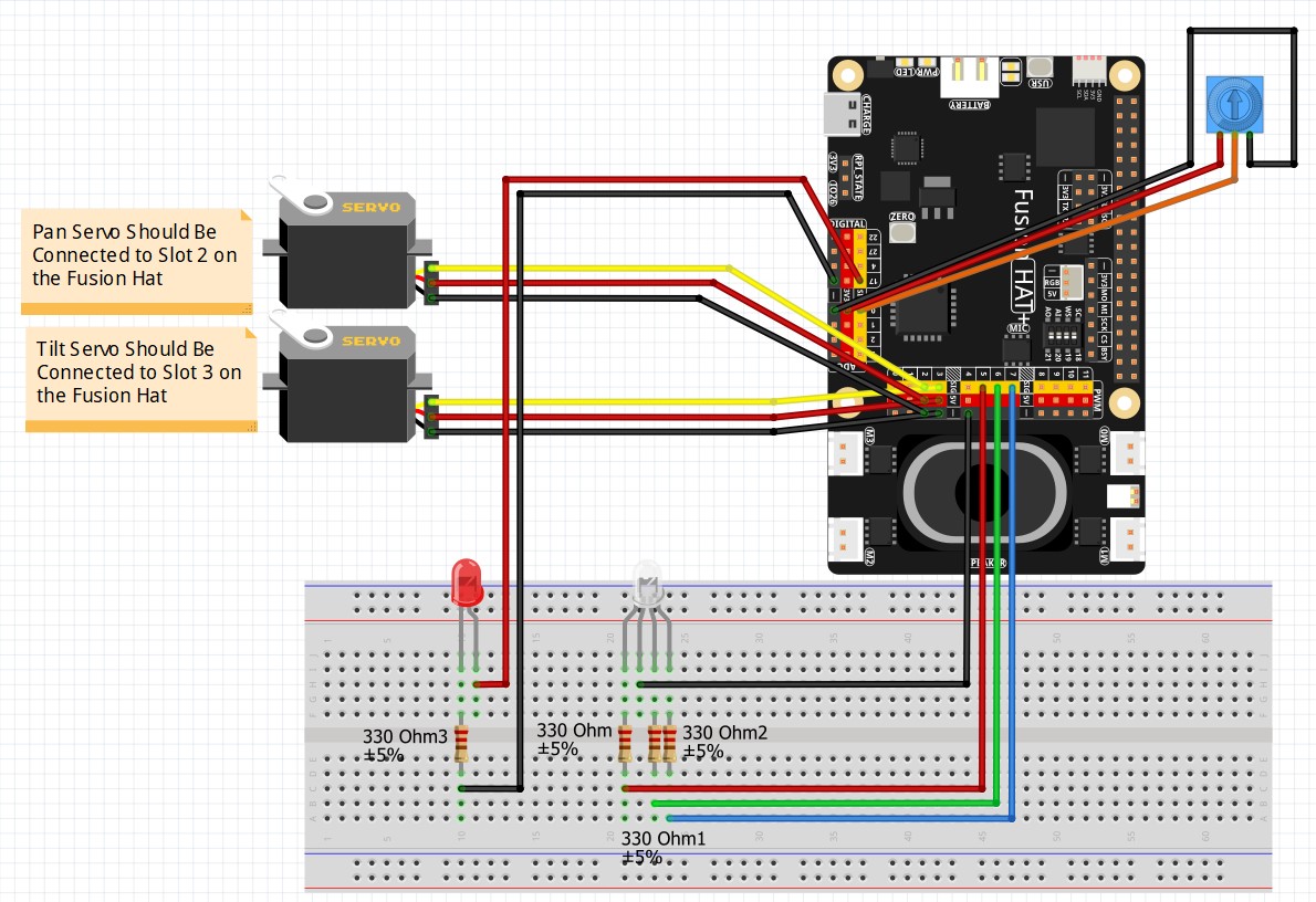
Fusion Hat Circuit Diagram
This is the circuit we will use moving forward in the class

This is the schematic to add the OLED:
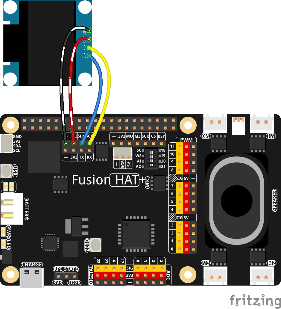
OLED
SSD1306 OLED Connected to the Fusion AI Hat

Then this is the schematic to add the NeoPixel
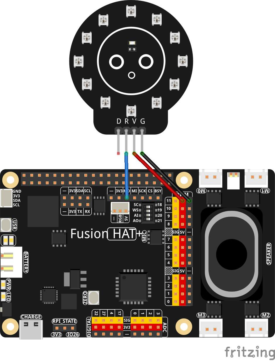
NeoPixel
NeoPixel Schematic

AI on the Edge LESSON 44: Displaying Live MediaPipe FaceMesh Avatar on SSD1306 OLED in OpenCV

This is Getting Crazy Cool!

Hey guys, welcome back to the Fusion AI Lab series, AI on the Edge! In Lesson 44 we just took things up another notch. We’re now running MediaPipe Face Mesh on our Raspberry Pi 5, pulling all 468 facial landmarks in real time, and then drawing a clean, smooth face contour directly onto a tiny 128×64 OLED display!

That’s right — your face is now living on that little monochrome OLED in real time! Every eyebrow raise, smile, head tilt, and eye movement gets faithfully reproduced on the display. We’re pulling the camera feed with picamera2, processing it with MediaPipe’s powerful face mesh, scaling the landmarks down to OLED resolution, and then drawing the official FACEMESH_CONTOURS connections using PIL. The result is surprisingly smooth and fun to watch! This project really shows the power of combining modern AI vision tools with simple embedded hardware. Watching your own face rendered in real time on a tiny OLED is just plain awesome — it feels like sci-fi stuff from just a few years ago, and now we’re doing it on the Edge with our Fusion AI Lab kit!

If you’ve been following along, you’re starting to see how powerful these tools are becoming. We’re no longer just detecting faces — we’re understanding the structure of the face and visualizing it however we want. And we’re just getting started!

So fire up your Raspberry Pi, grab that OLED, and let’s keep pushing the limits. You’re doing some seriously cool stuff!

In this lesson we are still using our standard Fusion AI Lab Kit cirtuit from the earlier lessons:

Fusion Hat Circuit Diagram
This is the circuit we will use moving forward in the class

We have also connected the OLED to the above circuit according to this diagram:

OLED
SSD1306 OLED Connected to the Fusion AI Hat

AI on the Edge LESSON 39: Understanding MediaPipe Data Structures

In this video lesson I show you how to understand the data structures returned by MediaPipe. I show you how to peel the data structure back, to get at the useful information.

When you run face detection with MediaPipe, the results object it returns is not a normal dictionary or list. It is a special custom object called SolutionOutputs. The easiest way to explore it is to start by checking the main attribute: results.detections. This is a Python list that contains one entry for every face detected in the current frame. If no faces are found, results.detections will be None or an empty list.

To extract useful information, you loop through results.detections. Each item in that list is a Detection object. From this object, you can access two main things: the confidence score using detection.score[0], and the location data using detection.location_data. Inside location_data, you will find relative_bounding_box (which gives you xmin, ymin, width, and height as values between 0 and 1) and relative_keypoints (a list of 6 facial points such as eyes, nose, and mouth).

The standard method is to first get the frame’s height and width, then multiply the normalized values (like xmin and width) by the actual pixel dimensions of the image to convert them into usable pixel coordinates. You can then use these coordinates with OpenCV functions such as cv2.rectangle() for the box or cv2.circle() for the keypoints.

By using simple print(type()), print(dir()), and print() statements on results, results.detections, and individual detection objects, you can quickly discover the full structure. This step-by-step approach — starting from results → detections → individual detection → location_data — lets you reliably reach all the useful information MediaPipe provides.

Below is the code we developed in the video.


AI on the NVIDIA Jetson Orin Nano: Adding Text-to-Speech (TTS) with Piper

In this lesson, we are building a local, offline voice pipeline using Piper. This engine runs natively on our Jetson Orin Nano hardware, providing fast and natural speech without needing an internet connection. To keep this simple, we will install everything into one specific folder so the software can easily find its own files.

Step 1: System Prep & Piper Installation

Open your terminal and run these commands one by one to create the workspace and download the required files. We are placing everything into the same directory to ensure the AI engine can always find the voice model.

Step 2: Identify Your Audio Device

Because every setup is different, we need to tell the system which speaker to use. Run the following command in your terminal:

Look through the list for your speaker. You will see something like card 0 and device 0. If your card is 0 and device is 0, your identifier is plughw:0,0. You will use these numbers in the Python script below.

Step 3: The Python Pipeline Script

Create a new Python file and paste the code below. Because we installed everything into the same folder, this script will find the files immediately.

Step 4: Customizing Your Voice

Piper has dozens of voices available. To see the full library, visit the Piper Voices Repository. Download the .onnx and .onnx.json files for your preferred voice, place them in the ~/voiceAssistant/piper/piper/ folder, and update the modelPath variable in your script.

Homework: The Talking Echo Bot

Your assignment is to play around with different voice models, and choose several that you like the best. Then modify the Python script so it becomes an interactive “Echo Bot.” Instead of hardcoding the message, use Python’s input() function to ask the user what to say. When the user types a sentence and presses Enter, your script should pipe that text into Piper and speak it back to you. Use a while True: loop to keep the program running so you can continue talking to your computer. Make a video of your working project, and the voices you chose.  In the description in your video, make sure to leave a link back to the video above. That way users can easily click between my video lesson over to your video, and then back to the class video.

No Cloud. No Internet. No Problem. Two Commands for Local LLM on Jetson Orin Nano

Hey guys, welcome back to the channel. Paul McWhorter here from TopTechBoy.com. Today, we aren’t just messing around with simple circuits or basic scripts—we are going to take that NVIDIA Jetson Orin Nano we rescued from the brink of destruction in the last video, and we are going to turn it into a completely sovereign, local thinking machine.

I don’t know about you, but I am tired of Big Tech telling me I need a credit card, a monthly subscription, and a constant high-speed internet connection just to make an AI model reply to a prompt. Today, we are going to do it completely naked. We are going to cut the cord, pull the ethernet, and run cutting-edge Large Language Models entirely on the local physical silicon of your Jetson Orin Nano.

And we are going to do it in exactly two commands. One to build the engine room, and one to fire up the mind.

Let’s get started.

The Hardware Architecture

Before we drop the code into the terminal, let’s understand exactly what we are building today. We are dealing with three core components working together in a unified system.

  • The Model (The Fuel): This is your raw neural network file (like Google Gemma or Meta Llama). It contains the weights, vocabulary, and potential intelligence. On its own, it’s just a massive, inert file sitting on your storage drive.

  • Ollama (The Engine Room): This is the heavy lifter. Ollama is a local execution framework that takes that raw model file and boots it directly into the Jetson’s unified RAM and CUDA cores. It handles the brutal mathematical calculations required to generate tokens.

  • The Terminal Chat (The Dashboard): This is your interface. It provides the clean command-line text box for you to type your prompts and prints the model’s responses back to you in real time.

The Two-Command Installation

Go ahead and fire up your Jetson Orin Nano, open a fresh terminal window, and get ready to type. Remember: copying and pasting makes you weak. Type these out like a real engineer so your hands learn the muscle memory.

Command 1: Install the Ollama Engine

This command fetches the official automated bootstrapper script from Ollama and executes it locally to configure the background system service on your host OS.

Command 2: Fire Up the Local Model

Once the installation script finishes, your engine room is live. Now, tell Ollama to pull down the optimized 1-billion parameter Google Gemma model and launch an interactive local dialog loop instantly:

The moment you hit enter, your Jetson will download the model weights directly to your local drive, load them straight into the VRAM, and drop you into a clean prompt box. Type a question, hit enter, and watch your local silicon generate answers with zero cloud dependencies.

Choosing the Right Mind for Your Machine

The beautiful part about setting up Ollama is that you aren’t locked into just one model. Different models have different parameter sizes and strengths. On the 8GB Jetson Orin Nano, you want to balance model size against your available hardware headroom to keep your generation speeds crisp.

Here are the verified, hardware-accelerated local models you can experiment with right out of the box:

Launch Command Model Family Size / Parameter Count Best Used For
ollama run gemma3:1b Google Gemma 3 1 Billion Ultra-fast responses, light footprint
ollama run llama3.2:1b Meta Llama 3.2 1 Billion High-efficiency conversational loops
ollama run phi4-mini:3.8b Microsoft Phi-4 3.8 Billion Heavy reasoning and coding logic
ollama run qwen3:4b Alibaba Qwen 3 4 Billion Structured data and multilingual logic
ollama run qwen3.5:4b Alibaba Qwen 3.5 4 Billion Advanced context processing
ollama run gemma3:4b Google Gemma 3 4 Billion Maximum analytical depth on Orin Nano

⚠️ Paul’s Engineering Note on Headroom

The 1B (1-Billion parameter) models are incredibly light and will run at lightning speed on the Orin Nano. If you want to push the machine harder for more complex reasoning, step up to the 3.8B or 4B models. Just keep an eye on your system resources—running a 4B model pushes close to the limits of the Orin Nano’s 8GB unified memory architecture, especially if you are running a heavy graphical desktop environment in the background!

To exit out of any active terminal chat session and return to your standard command prompt, simply type:

Homework Assignment

Alright, you have the hardware running, you have the engine installed, and you know how to switch out the minds of your machine. Now it’s time for your homework.

I want you to install both the gemma3:1b model and the heavier gemma3:4b model on your Jetson Orin Nano. Run them both through a test sequence: ask them to write a simple Python script, and then ask them a complex logic riddle.

I want you to observe the difference in quality of thought versus speed of generation. Is the 4-billion parameter model smart enough to justify the extra computation time on your hardware, or does the 1-billion parameter model give you the snappy responsiveness you need for a real-time edge application?

Leave a comment down under the video showing your results, tell me which model you prefer running natively on your bench, and I will see you guys in the next lesson!